The =offset() function is the "ace up my sleeve" when building real estate financial models. Site visitors and folks who frequently use Tactica's free and paid Excel workbooks will often comment on the repetitive use of the offset function. 

If you're not used to this Excel formula, following the logic and understanding its purpose can be challenging. I plan to detail how the function works and its best uses in a financial modeling context.

This article is a must-read if you strive to learn Microsoft Excel or improve your financial modeling abilities. If you’re using a Tactica model, the knowledge will prove helpful when interpreting the formulas within your proforma. This blog post will serve as an Excel tutorial of sorts.

Excel Offset Function Contents

1. Excel Offset Function Syntax

2. Excel Offset Formula Syntax Examples

3. Offset Excel Formula Best Uses

   • Data Presentation

   • Data Aggregation

   • Dynamic Charts

4. Video: Simplifying the Offset Formula in Excel

Below are the arguments you need to populate the offset formula:

=OFFSET(reference cell, rows, cols, [height], [width])

Note: You won't be required to use all assumptions in many instances. If this is the case, you can leave it blank. Height and width are [optional arguments].

For example, if you only want to reference cell A1 and use the "rows" argument, you'd populate the formula as:

=OFFSET(A1, 2 , , , )

The best way to show you how the offset formula works is with examples.

You'll always need a reference cell. Below, I have a range of cells with random numbers:

Let's show a few examples of using the offset formula.

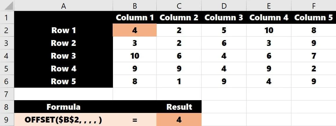
In the first example, let's only populate the reference cell (B2) and leave all other arguments blank.

=OFFSET($B$2, , , , )

It's pretty simple; the offset formula references cell B2 and returns the value in that cell (4).

Note: I am locking the reference cell (B2) as this will always be the reference.

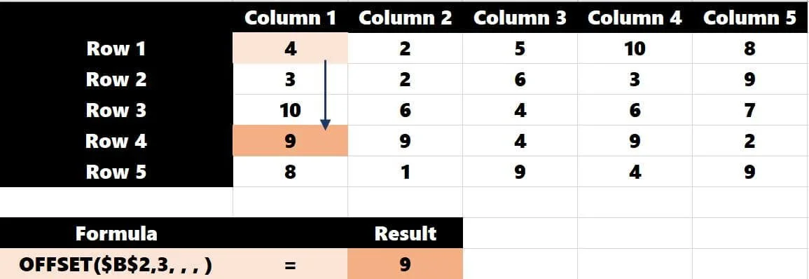
Now, let's populate the row argument. The specified number of rows below the reference cell = 3.

=OFFSET($B$2, 3 , , , )

The returned reference is "9," three rows below cell B2.”

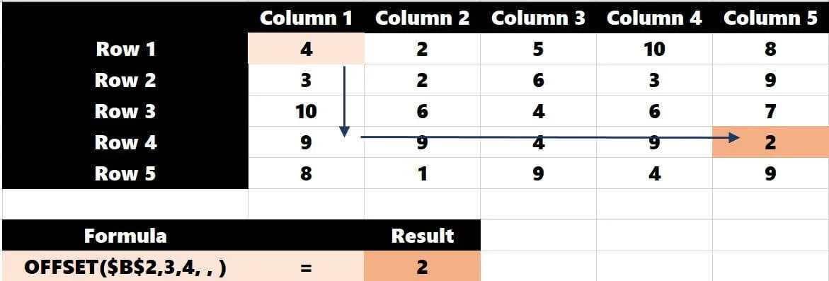
Let's go one step further and add a column cell reference. This will specify the number of columns to reference to the right of the reference cell.

=OFFSET($B$2, 3 , 4 , , )

Now, Excel will count down three rows from the reference cell and four columns to the right.

The returned range is the "2."

The last two arguments are "height" and "width." We will cover these arguments when we discuss the best uses. The row and column arguments would be sufficient if you need to reference a single cell.

Note: I am using positive numbers for row and column arguments in the above examples. You could also use negative numbers if you want to go “up” and the “left” of the reference cell instead of “down” and to the “right"””

You may ask yourself, how does this help with financial modeling? Let's get into the Excel offset function’s best uses.

There are three consistent offset uses in Tactica underwriting models.

Formatting data is essential for presentation. Sometimes, data is best presented vertically for one aspect and horizontally for another.

For example, you have a worksheet that hosts the amortization table for the financing. This data is presented vertically.

However, on the "Returns Summary" tab, you want to horizontally present the debt service payment data. 

Offset is the perfect solution to seamlessly capture the loan paydown data from another tab. For simplicity, I have the amortization table and the loan payout on the same page, so it's easier to follow the formula.

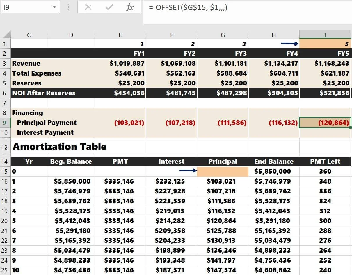
Here is the offset formula for principal payments.

=-OFFSET($G$15, E$1, , , )

This first principal payment is grabbing the $103,021 directly, one cell below the reference cell (G15).

I can then drag the formula to the right to populate the other columns.

My "number of rows" argument is dynamic and moves with the columns. For example, when we look at the formula in Year 5, the row reference is "5", and Excel pulls the entry five rows below the reference cell (G15) in the amortization table ($120,864).

The formula for interest payments is nearly identical except for the reference cell (now it’s above the interest column).

=-OFFSET($F$15,E$1,,,)

I would drag this formula to the right as I did with the principal payments. Offset is a very efficient formula to look up data on another tab that must be presented differently, like the examples above.

Adding a "sum" formula to "offset" opens up another world of opportunities. Often, several columns need to be added together, and offset offers the perfect solution.

You will see this combination frequently in the Tactica model. Here is an example of how Sum(Offset) is used in the Redevelopment Model.

The redevelopment analysis starts at a very granular level, down to the individual units and their monthly rent. I use the =sum(offset()) formulas to take and annualize this monthly data.

Below, I am looking at only the first-floor units. The average rent per unit is $1,199 for Months 1-12.

Below that grid, we have the annualized totals for the first-floor units. This is where we use the offset formula.

=SUM(OFFSET($E291, ,(D$374 - 1)*12, ,12))

Let’s ignore the *$D$72 for the time being.

Let's break down this formula and discuss what each section is doing. 

Reference Argument = E291 is the starting reference.

Row Argument = None

Cols Argument = ( 1 - 1 ) x 12 = 0

Height Argument = None

Width Argument = 12

This is the first time we've discussed the width argument. Because we are annualizing the monthly data, an entry of 12 tells Excel to grab 12 columns (months) from the cols argument cell (which in this instance is “0” and defaults to the Reference Argument). Below is what offset is selecting:

Cell D72 = eight units, so the 12 months of average rents are multiplied by 8

$1,199 x 12 x 8 = $115,092

Let's look at the offset formula one column over.

=SUM(OFFSET($E291, ,(E$374-1)*12, ,12))*$D$72

Reference Argument = E291 is still the starting cell

Row Argument = None

Cols Argument = ( 2 - 1 ) x 12 = 12

Height Argument = None

Width Argument = 12

The only change is that the "Columns Argument" begins 12 cells over from the reference cell (the 13th cell). Now the Sum(Offset) formula is totaling Monthly 13 - 24.

13th cell = Stipulated by the Column Argument (the new starting point).

Columns 13 - 24 = Stipulated by the Width Argument (12 columns)

Once you correct the offset formula, you can drag the formula over the desired range of adjacent cells.

Note: Locking cells is crucial and makes dragging formulas possible and efficient.

Another superb use for the offset function, specifically, dynamic charts.

I tackled this in another article (video tutorial included): Automating Excel Charts with the Offset Function.

Summarizing Offset Function in Excel

Reference functions like the offset can enable more efficient analysis in your Excel workbook. I gave you two examples of using this formula in a real estate modeling scenario. Another blog post covers how to unleash the offset formula on your charts to ensure graphics are updating automatically as your data inputs change.

A direct cell function (= cell) may work in the short term and be a more straightforward solution. However, the offset function is how Excel pros reference cell(s) and ensure longstanding precision and accuracy in a changing workbook environment with vast inputs.

Tactica uses the offset function consistently for:

• Superior data presentation

• Data aggregation

• Dynamic charts & graphics

Learning the offset syntax and its best uses is an absolute game-changer if you spend much time in Microsoft Excel.